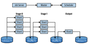
BigQuery High-Level Architecture

Query Step
Step 1: HTTP POST
The client sends an HTTP POST request to the BigQuery endpoint. Usually it use JDBC

Step 2: Routing
The part of URL indicated which cloud project is responsible for paying for the request. If you project has configured the location, the query will be routed. Otherwise, the router must parse the query to determine what datasets are involved. Datasets are tied to locations.
If your query don’t have dataset, then it will default to send to US.
Step 3: Job Server
The BigQuery Job Server is responsible for keeping track of the state of a request. The job server performs authorization to ensure that the caller is allowed to run a query. The job server is in charge of dispatching the request to the correct query server.
The BigQuery must understand the capacity of various compute and storage clusters, network topology, availability zones and where the data currently exists. Then BigQuery can rebalance the data and optimize future query.
When backup or failover processes happen, BigQuery will triggers a train, or failover, of a computer cluster on the order of once per week. Drains can happen for network failure, degradation of service or unusually high queue length. Other jobs will switch to secondary cluster.
Step 4: Query Engine
Query is routed to a Query Master, which is responsible for overall query execution. Query master contacts the metadata server to establish where the physical data resides and how it is partitioned. Then Query Master requests slots from the scheduler. One slot generally represents hals of a CPU core and about 1GB of RAM.
Step 5: Returning the query results
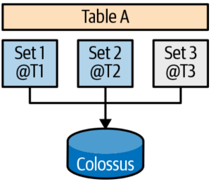
Results have two parts. They first page is stored in Spanner along with the query metadata. Spanner data is located in the same region in which the query is running. The remaining data is written to Colossus.
Some query may need lots of time to run. Before connection time out, BigQuery will return a job id. Client can get results by looking up that job to get the results.
Result will be reserved for 24 hours and limited to 10GB. You should write to a table if the result is important.
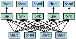
Query Engine Dremel
Dremel start with a static tree structure for execution plan. Tree structure works fine for scan-filter-aggregate queries. But it need several visits for query involve join. Dremel X builds a dynamic query plan that can be any number of levels and can even change the plan while the query is running.
Dremel has three parts: the Query Master, the Scheduler, and the Worker Shard.
Query Master
Responsible for query parse. It have column prune. Then it will connect to meta-server with a special meta-file. Meta-file shows locations of files within the table and how they map to field values. Query master will run another Dremel query against meta-file
Scheduler
It is responsible for assigning slots to query. A slot is a unit of work that generally corresponds to the processing of a single file or shuffle sin for later stages. A query that processes a petabyte of data might use 10 million total slots. The resources will be gradually assigned during query.
On demand user can use up to 2000 slots to run query. If not enough slots are available, the scheduler will reduce all on-demand users' slot allocation proportionally. Scheduler will use a 'fair' approach to allocate resources. Scheduler will cancel running slots at any time to make way for a user with higher priority or to ensure fairness. The reversed slots are arbitrarily. User can get these resources any time they want.
Worker Shard
The Worker Shard is responsible for actually getting the work done in a query. A Worker Shard is a task running in Borg, Google's container management system. The destination location is usually an in-memory filesystem. The in-memory filesystem provides short-term durable storage between stages of the query.
Shuffler
The number of shards involved in a stage is largely dependent on the number of shuffle sinks that were written. BigQuery will dynamically change the number of shuffle sinks during a query depending on the size and shape of the output. The BigQuery will spill data to disk too.
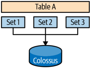
Storage
Colossus have erasure encoding, which means that it stays durable even is a large number of disks fail or are destroyed. Write data multiple times is called encoding in Colossus.
The simplest type of encoding is called replicate encoding.
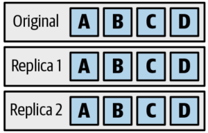
Replica is expansive. To store less data, many distributed filesystems use something called erasure encoding or Reed-Solomon encoding. Erasure encoding stores mathematical functions of the data on other disks to trade off complexity for space.

Erasure encoding, in which extra "encoded" data can be used to recover data in the event of a failure of any of the original chunks of data. Erasure encoding will slow down read. If the primary copy is no response, we need extra reads to start a recovery read.
Capacitor is the second generation of format used within BigQuery; the first was a basic column store. One of the key features of Capacitor is dictionary encoding. That is, for fields that have relatively small cardinality (few distinct values), it stores a dictionary in the file header.
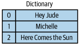
For example a reasonable small popular music can be played. The dictionary will store in file header. Instead of storing the full tile, Capacitor can just store the offset into the dictionary, which is much more compact.
The first column is the encoded song title, and the second column is another data field (perhaps the customer who requested that the song be played).
Filter can be pushed on the header sometime.
To further save on space, Capacitor does run-length encoding. That is, if the value "2" appears five times in a row, you can store "2:5". For long runs of the same value, this can give significant compression.
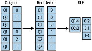
Capacitor employs a clever trick - it simply reorders the rows to obtain a compact encoding. Rows in BigQuery are not ordered, and there is no guarantee or even expectation of which rows come after which other rows. Because computing the best ordering is an NP-hard problem, BigQuery applies a set of heuristics that gives good compaction but runs in a short amount of time.
Metadata
Metadata is data about the data that is stored. Metadata includes entities like schema, field sizes, statistics, and the locations of the physical data. Many of the limits that BigQuery imposes, like the number of tables that can be referenced in a query or the number of fields that a table can have, are due to limits in the metadata system. BigQuery table metadata has three layers. The outer layer is the dataset, which is a collection of tables,, models, routines, and so on with a single set of access control permissions. The next layer is the table, which contains the schema and key statistics. The inner layer is the storage set, which contains data about how the data is physically stored.
Storage sets
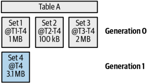
A storage set is an atomic unit of data, created in response to a load job, streaming extraction, or Data Manipulation Language (DML) query. Storage sets enable updates to BigQuery tables to be ACID compliant. The underlying physical storage for BigQuery is immutable. Storage sets generally go from Pending -> Committed -> Garbage.
Time Travel
BigQuery supports time travel for seven days in the past. To enable time travel, BigQuery keeps track of the timestamp at which storage set transitions happen.
Storage optimization
When you are writing or updating data over time, storage can often become fragmented. The storage optimizer helps arrange data in to the optimal shape for querying. It does this by periodically rewriting files (LSM tree like way).
Partitioning
Partition is essentially a lightweight table. Partitions have a full set of metadata and physically separate location from other partitions. If you need higher cardinality, you should use clustering. One way of reducing the number of partitions is to create a separate field that truncates the event date to the month level and partitions by that field. BigQuery uses storage sets that are marked with the partition ID. This makes it easy to filter based on partitions.
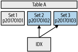
IDX is a Spanner database index that helps us find only the storage sets within that range.
Clustering
Clustering is a feature that stores the data in semisorted format based on a key that is built up from columns in your data. It can do a binary search to find the files at the beginning and end of the range.
The data files have headers that contain the min and max values of all the field. The advantage here is that it allows you to check whether a value is in the table just by looking at the header. Note the data isn't sorted within one file. Data in Capacitor files is reordered to improve compression ratios.
If you add new row into BigQuery table with clustering. BigQuery will generate new file for new rows according to rows range. The original files are immutable. BigQuery need to recluster data after a while. BigQuery maintains a clustering ratio, which is the fraction of the data that is completely clustered.
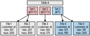
In T2, set1 and set2 were overlapped. In T3, reclustering happend.
Optimizing Performance and Cost
We should be caution that performance tuning should be carried out only at the end of the development stage. You can query the INFORMATION_SCHEMA table to get the most expansive queries. The most important three parts are:
- How much data is read and how that data is organized
- How many stages your query requires and how parallelism those stages are
- How much data is processed at each stage and how computationally expensive each stage is
Example Query:
SELECT
   job_id
   , query
   , user_email
   , total_bytes_processed
   , total_slot_ms
FROM `some-project`.INFORMATION_SCHEMA.JOBS_BY_PROJECT
WHERE EXTRACT(YEAR FROM creation_time) = 2019
ORDER BY total_bytes_processed DESC
LIMIT 5
The work loader tester requires Gradle. Followings are some suggestion for optimization:
- Minimizing I/O
- Caching the results of previous queries
- Performing efficient joins
- Avoiding overwhelming a worker
- Using approximate aggregation functions
BigQuery can use create or replace MATERIALIZED VIEW to materialized query. When a query is re-run and a materialized view exists, the query doesn't need to rescan all the table again. All incremental data changes from the base tables are automatically added to the materialized views.
BigQuery will auto save cache for 24 hours. But the query need to be exactly matched. Queries are never cached if they exhibit nondeterministic behavior (for example, current timestamp or rand), if the table changed, if the table is associated with a streaming buffer, if the query uses DML statements
Performing Efficient Joins
Denormalization like create a temp table for cache redundant data. It will increase data volume, but it can boost query (need to balance). Avoiding self-joins of large tables.
BigQuery can use APPROX_* (quantiles, count, top_count) to get approximate result. It works better on large scale data.
Otherwise, BigQuery can use HLL algorithm by following three procedure
- Initialize a set, called an HLL sketch, by adding new elements to it by using HLL_COUNT.INIT
- Find the cardinality of an HLL sketch by using HLL_COUNT.EXTRACT
- Merge two HLL sketches into a single sketch by using HLL_COUNT.MERGE_PARTIAL.
In addition, HLL_COUNT.MERGE combines steps 2 and steps 3.
Optimizing How Data is Stored and Accessed
Data should be located in the same region of GCP to accelerate calculation.
You can set compressed and partial response to minimize network overhead. Accept-Encoding: gzip User-Agent: programName (gzip)
BigQuery is better to use internal storage. If you want to use external storage, please use a compressed, columnar format.
Create a life cycle management for BigQuery.
Array aggregation is a cost operation. If you want to use the same array several times. Array of Struct will be better.Array of Struct can help in reducing duplicate non struct properties. A key drawback to nested, repeated fields is that you can not easily stream to this table.
ST_GeogFromText can help in geo format calculation. This is also a trade off too. It is better for scenario like one time calculation and many queries.
Clustering, like partitioning, is a way to instruct BigQuery to store data in a way that can allow less data to be read at query time. Clustering can be done on any primitive non-repeated columns. When you cluster by multiple columns, you can filter by any prefix of the clustering columns and realize the benefits of clustering.
MERGE and DML command can re-clustering the table.
| Partitioning | Clustering | |
|---|---|---|
| Distinct values | Less than 10,000 | Unlimited |
| Data management | Like a table (can expire, delete, etc.) | DML only |
| Dry run cost | Precise | Upper bound |
| Final cost | Precise | Block level (difficult to predict) |
| Maintenance | None (exact partitioning happens immediately) | Background (impact might be delayed until background clustering occurs) |
If other column is correlate to clustering columns, BigQuery can reduce reading too. Clustering column join will have parallel optimization.
SELECT o.*
FROM orders o
JOIN customers c USING (customer_id)
WHERE c.name = "Changying Bao"
If the order table is cluster by customer id. Then the query will be optimized:
// First look up the customer id.
// This scans only the small dimension table
SET id = SELECT customer_id FROM customers
WHERE c.name = "Changying Bao"
// Next look up the customer from the orders table.
// This will filter by the cluster column,
// and so only needs to read a small amount of data.
SELECT * FROM orders WHERE customer_id=$id ;
The order table can reduce reading.
BigQuery can set batch flag which allow queue buffer and retry.
The data doesn’t change for 90 days, the cost will be reduce. If these data doesn’t change, please don’t use DML query.
WITH clause is effective. It can improve readiness and cache intermediate query.
UDF example
CREATE TEMPORARY FUNCTION dayOfWeek(x TIMESTAMP) AS
(
  ['Sun','Mon', 'Tue', 'Wed', 'Thu', 'Fri', 'Sat']
      [ORDINAL(EXTRACT(DAYOFWEEK from x))]
);
CREATE TEMPORARY FUNCTION getDate(x TIMESTAMP) AS
(
  EXTRACT(DATE FROM x)
);
CREATE OR REPLACE FUNCTION ch08eu.dayOfWeek(x TIMESTAMP) AS
(
 ['Sun','Mon', 'Tue', 'Wed', 'Thu', 'Fri', 'Sat']
    [ORDINAL(EXTRACT(DAYOFWEEK from x))]
);
If you want to query certain offset from an array. Need to add UNSET:
SELECT pay_by_quarter[ORDINAL(3)] FROM sal_emp, UNNEST(pay_by_quarter)
Array function: ARRAY_AGG, GENERATE_DATE_ARRAY, ARRAY_CONCAT, ARRAY_TO_STRING
Window function: Similar to Spark. BigQuery support PARTITION BY,  ORDER BY and ROWS BETWEEN $(NUM} PRECEDING AND ${NUM} PRECEDING syntax. Function like AVG(*), RANK(), LAST_VALUE(*), LEAD(*)
Time Travel:
Query 6 hours ago data example
SELECT
  *
FROM `bigquery-public-data`.london_bicycles.cycle_stations
FOR SYSTEM_TIME AS OF
    TIMESTAMP_SUB(CURRENT_TIMESTAMP(), INTERVAL 6 HOUR)
MERGE statement is an atomic combination of INSERT, UPDATE and DELETE operations that runs as a single statement. MATCH statement can help in different operation scenarios.
MERGE ch08eu.hydepark_stations T
USING
  (SELECT *
   FROM `bigquery-public-data`.london_bicycles.cycle_stations
   WHERE name LIKE '%Hyde%') S
ON T.id = S.id
WHEN MATCHED THEN
   UPDATE
   SET bikes_count = S.bikes_count
WHEN NOT MATCHED BY TARGET THEN
   INSERT(id, installed, locked, name, bikes_count)
   VALUES(id, installed, locked,name, bikes_count)
WHEN NOT MATCHED BY SOURCE THEN
   DELETE
You can write a script and save it to a procedure.
CREATE OR REPLACE PROCEDURE xx.xx(${parameter}) BEGIN -> END